Making Waves in Arrays

Background

Forty years ago, I read a paper and … This would have been too cheesy to start with. Anyways:

I first read about systolic arrays 40 years ago. I was looking for a topic to write a term paper during the last semester of university and flipping through recent IEEE Computer editions, I found H.T. Kung’s seminal paper titled Why Systolic Architectures? Its arguments about how special-purpose systems should be designed made perfect sense to me. Especially calling for simple/regular designs, focusing on concurrency instead of faster clock and most importantly balancing computation with I/O speed all made sense. I remember reading the article over and over to see the beauty in simplicity to perform complex operations such as Fast Fourier Transform (FFT), convolution or matrix multiplication concurrently.

Before, we look at what a systolic array is, let’s choose an operation and remember how it is computed. For my learning exercise, I decided to use matrix multiplication. Matrix multiplication is a foundational operation that powers numerous technologies that we rely on today including signal processing (yes, that mobile phone or notepad where you may be reading this), web search algorithms such as PageRank, graphics and rendering (to rotate, transform, scale objects), simulations of bridges, proteins, climate, etc. Last but not least, I can tell you that if dreams of Artificial General Intelligence become a reality one day, it will be because of matrix multiplication. More on that later!

Just to remind ourselves about how matrix multiplication works:

• $A$ is an $m × n$ matrix and $B$ is an $n × p$ matrix

• The matrix product $C = A*B$ is defined to be the $m × p$ matrix

• where $c_{ij} = \sum_{k=1}^{n} a_{ik}b_{kj}$ for $i = 1, ..., m$ and $j = 1, ..., p$

In terms of complexity, since the resultant matrix has $mp$ elements and each element has $n$ multiplications (and $n-1$ additions, but we can neglect the cost of additions), the total amount of multiplications is $mpn$. For the sake of simplicity, if we use square input matrices, i.e., if both A and B are $n × n$ dimensions, then the complexity of a matrix multiplication is $O(n^3)$.

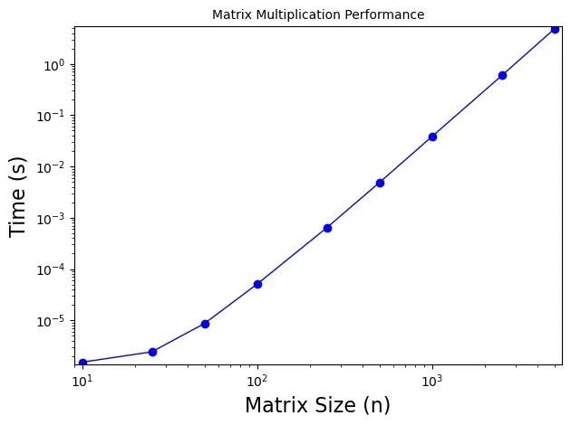
Today if you happen to perform a matrix multiplication operation on a traditional computer such as your laptop or phone, you will be ending up spending $n^3$ time. Just to confirm the complexity, I ran a benchmark of square matrices from 10x10 to 5000x5000 (anything bigger ends up risking the depletion of the computer memory) and ended up with the following figure. The plot is drawn at $loglog$ scale to show the linearity of the cost. It also shows that at small matrix sizes, the addition operation has some influence on the overall time matrix multiplication takes. However, as we move to higher matrix sizes, almost all the time ends up being spent on multiplication.

There is a very active mathematics research area around how to optimize matrix multiplication. The first breakthrough in this quest was made by Volker Strassen in 1969 when he showed that two $2x2$ matrices can be multiplied by performing 7 instead of 8 multiplications. His algorithm is a marvel where he reduces the number of multiplications by performing more additions (and subtractions). Then more importantly defines how to partition large $nxn$ matrices into $2x2$ and take advantage of his algorithm. I recommend reading the Wikipedia page that describes Strassen algorithm to understand its ingenuity. After Strassen’s first discovery, the research on such optimization has continued to this day where the objective is to reduce the matrix multiplication complexity from $O(n^3)$ to $O(n^2)$. Strassen managed to bring this to $O(n^{log_{2} 7})$. These days the best algorithm is at $O(n^{2.371339})$. Ironically, today many researchers are using machine learning tools that rely on matrix multiplication in their pursuit of matrix multiplication optimization. If you are interested, check out multiple articles appeared in Quanta magazine lately.

Even if the ultimate pursuit of $O(n^2)$ is achieved, matrix multiplication is a very costly operation, especially considering how frequently it needs to be performed for various applications that I mentioned earlier. That brings us to the 40-year old paper about systolic architectures that are tailored for such operations by relying on a large number of computing units (also known as processing elements). The first essential feature of a systolic architecture is the simplicity of its processing element (PE) design. This is easily fulfilled for a matrix multiplier systolic array since the operation step called multiply-accumulate (MAC) is very simple. It is:

Using the MAC step iteratively, i.e., for successive $n$ pairs of $(a_{ik},b_{kj})$ where $k = 1,..,n$ we can compute the value of $c_{ij}$. Next step in the systolic architecture design would be to perform multiple operations concurrently. That means at a given time multiple PEs would be performing MAC operations towards calculating the value of corresponding resultant matrix element $c_{ij}$. By extending the number of PEs to $n^2$ it is possible to increase the number of concurrent MAC operations to its maximum. The most important part of the systolic architecture design is as the name implies, the movement of input data from PE to PE similar to the heart muscle’s contraction to pump blood. Similar to the systolic beat, synchronized with a clock, input matrix elements move from one PE to another and used in each PE for the MAC operation.

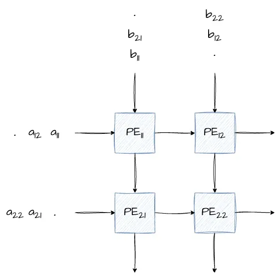
Easiest way to explain a systolic array is to draw one. Following is a simple diagram of a 2x2 systolic array that can be used for matrix multiplication. In this diagram:

• Each PE is a simple unit that performs register $\leftarrow$ register + input(left)*input(top) and passes the input to its output ports, i.e., output(right) <- input(left) and output(bottom) <- input(top)
• As shown in the diagram, elements of the input matrices A and B are fed in a skewed pattern so that the right input matrix element arrives at the right PE at the right clock time.

We can describe the systolic array using uniform recurrence equations. For a matrix multiplication $C = A * B$, the formal specification $S$ is:

where $a(i,j,k) = a(i,j-1,k)$ and $b(i,j,k) = b(i-1,j,k)$ and remembering the matrix multiplication definition: $c_{ij} = \sum_{k=1}^{n} a_{ik}b_{kj}$ Using the formalism we can know when and where the resultant matrix element $c_{ij}$ is computed in the systolic array:

• Computation location: $l = (i,j)$
• Computation completion time: $t = i + j + k - 2$

Above formula also allows us to figure out how many systolic beats (cycles) it would take to compute the matrix multiplication. Considering the maximum values for $i,j,k$ is $n$ for $nxn$ square matrices, that means the last element $c_{nn}$ will be completed at $t = 3n - 2$. In other words using $n^2$ PEs we can complete the multiplication of two $nxn$ matrices in $3n-2$ steps instead of $n^3$.

Matrix multiplication (as well as many other linear algebraic operations) is at the heart of many machine learning neural networks. Starting with Recurrent Neural Networks, following with Long Short Term Memory and Gated Recurrent Unit; and ultimately with Transformer we see the heavy usage of matrix multiplication. This triggered hardware vendors such as Nvidia with GPU Tensor cores and Google with tensor processing units (TPUs) incorporating systolic arrays into their machine learning optimized hardware. In case of Nvidia array sizes are typically small (4x4 to 16x16) whereas Google decided to adopt higher degrees of parallelism with quoted values of 128x128 systolic arrays. I plan to learn to write more about how matrix multiplication as well as other linear algebra techniques are used in various neural network architectures in the future.

Focus of Learning

Let me outline my objectives in terms of learning quickly:

• My ambition was to build a systolic array simulation
• Use Kubernetes for the distributed system implementation since it provides all the essentials for orchestration and networking
• Specifically use indexed Jobs that would implement PEs
• Use an HTTP API to communicate with the PEs as well as for their inter-communication

That meant the following tasks need to be completed to build the systolic array simulation:

1. Create a Docker image that would be used as the Job’s image corresponding to a PE
2. Create a Docker image that would be used as a Deployment that orchestrates the Job pods by feeding input matrices to and collecting results from the PEs, providing a clock for synchronization and a user interface for the simulator user
3. Develop a set of Kubernetes definitions that would implement the PE Job, the Orchestrator Deployment and a headless Service for inter-PE as well as orchestrator-PE communication

In order to shorten the time for code development, I ended up using ChatGPT 5.2 for the majority of tasks 1 and 2 that I outlined above. I fed it with the following prompts:

__ASK__: build a NxN systolic array for matrix
multiplication as a demonstration of Kubernetes
indexed jobs communicating via a headless service.
__CONTEXT__: use a fastAPI based base image to
communicate among pods belonging to Jobs. use the
job index number to select the right pod for communication 
__CONSTRAINTS__: receive the input arrays, A and B
in a systolic way, entering from the left (A) and
from the top (B). assume the input matrices are both NxN
__EXAMPLE__: when all calculations are done for
multiplication and additions in 3N-2 steps, retrieve
the results from all systolic array elements via an
external reader using an API; here is a sample response
from the REST API.

After a small number of iterations between ChatGPT and I, the code started working as a collection of processes in my development environment. Then ChatGPT retrofitted it to running in Docker. Once that became operational, I developed the Kubernetes manifests.

Implementation Details

In order to follow the rest of the blog, please check the GitHub repository blog-making-waves.

Create a Container Image for Systolic Array Processing Element

This container image is implemented in Python using primarily FastAPI and httpx.async for asynchronous HTTP communications among PEs. Follow the instructions in the README file for the GitHub repository systolic-pe to build and store the image.

Probably the most relevant part of this implementation is the use of JOB_COMPLETION_INDEX environment variable to calculate the PE indices $i, j$ and use of a headless service to communicate among pods belonging to the Job as well as allowing the orchestrator to access the pods.

Create a Container Image for Systolic Array Orchestrator

This container image is implemented in Python using primarily FastAPI and httpx.async for asynchronous HTTP communications with PEs to feed data and collect their status so that it can be represented on a user interface. It also includes a basic UI that relies on server sent events to show the state of each PE at every tick (systolic pulse). Follow the instructions in the README file for the GitHub repository systolic-orchestrator to build and store the image.

Deployment of the Kubernetes Resources

Assuming you happen to have access to a Kubernetes cluster, follow the instructions of the GitHub repo blog-making-waves to simplify the generation of resource files. I’d recommend you use the demo deployment option using kustomize.

Complete the following steps for customization:

1. Create a namespace demo in your cluster.
2. Update $CONTENT/overlays/demo/kustomization.yaml to add the namespace and point to your container image registry for systolic-pe and systolic-orchestrator.
3. Update $CONTENT/overlays/demo/making-waves-demo.env, primarily to set the array dimension $N$.
4. Update $CONTENT/overlays/demo/systolic-pe-job-patch.yaml to set the Job completions and parallelism values to $N^2$.
5. Run kubectl apply -k $CONTENT/overlays/demo to deploy all the resources.

You will be able to access the UI at http://<NODE_IP>:<UI_NODE_PORT>/ui. Using the UI, you can increase/decrease the tick period and more importantly change the input matrices A and B. In my resource limited Kubernetes cluster, I ran 36 (6x6) PEs and the systolic array performed very well. Here is a video for a 4x4 array.

<!-- Fallback text for browsers that do not support HTML5 video -->
Your browser does not support the video tag.

Blog’s lead image was generated from plotting $sin(\frac{3x}{2}+\frac{y}{2}+t) + sin(\frac{6y}{5}+t)$ for t between 0 and $2\pi$. Inspiration comes from Square Waves.