Background

The first time I saw the word transcendental in a math book, I couldn’t figure out its significance considering I had associated the word in my mind with yoga poses or meditation hums. The word originated around 1600s to signify spiritual or supernatural … (that I hesitate to fill). The first recorded use of the term transcendante (not sure if in a French or Latin paper) was by Leibniz when he proved that $f(x) = sin(x)$ is not an algebraic function of x. In other words, it is not possible to find $p_{0}(x), p_{1}(x), ...$ such that

$p_{0}(x) + p_{1}(x)f(x) + p_{2}(x)f^2(x) + ... = 0$

After three quarters of a century, in 1748 Euler called trigonometric functions as transcendental quantities that arise from the circle. More importantly, he conjectured that if $log_{b}a$ is irrational, it is also transcendental. In 1761, Lambert conjectured that both $e$ and $\pi$ are transcendental numbers. Starting around mid-1850s, the research around transcendental numbers picked up. First Hermite proved $e$ being transcendental in 1873. Then in 1882 Lindemann proved the same for $\pi$ relying on the most beautiful mathematical equation, Euler’s identity ($e^{i\pi} = -1$) and put an end to the famous problem of Squaring the circle as proposed by the ancient Greeks.

Transcendental nature of $\pi$ has attracted a lot of people to figure out how to compute it with increasing accuracy starting with ancient Egyptians, Babylonians and Sumerians. The famous approximation $\frac{22}{7}$ we are familiar with first appeared in Archimedes’ treatise Measurement of a Circle in 250 BC. Another +700 years had to pass for Chinese astronomer Zu Chongzhi to discover the lesser known but a significantly better approximation $\frac{355}{113}$. It took more than 8 hours of mainframe time to compute the first 100K digits in 1961, while the same feat took almost a day in 1973 for 1M digits. More recently thanks to very high capacity memory modules, $\pi$ calculation has turned into a computer storage benchmarking exercise.

• In 2022, Google has published their feat of calculating 100T ($10^{14}$) digits which took 158 days on a cloud instance along with a 663TB temporary storage disk + 100TB to store the finally computed digits.
• In November 2025, StorageReview achieved the calculation of 314T ($3.14*10^{14}$) digits after 110 days on a dedicated hardware with a Dell PowerEdge R7725 (1.5TB RAM) and 2.4PB of storage.

All of these high performance computing exercises have become possible thanks to the discovery of very rapidly converging algorithms to calculate $\pi$. To keep the story short, there are two notable algorithms:

1. Gauss-Legendre algorithm that relies on the convergence of arithmetic and geometric means (AGM) of two positive real numbers to the same value. $\pi = \frac{4*AGM(1;1/\sqrt{2})}{1 - 2*\sum_{j=1}^{N} 2^j*c_{j}}$ where

   $a_{n}=\frac{a_{n-1}+b_{n-1}}{2}$, $b_{n}=\sqrt{a_{n-1}b_{n-1}}$, $c_{n}=a_{n}^2 - b_{n}^2$

Lorenz Milla gives a proof that can be followed with basic understanding of calculus. Algorithm converges quadratically that allows doubling the number of accurate digits with each step of computation.

2. Chudnovsky algorithm that relies on the famous Indian mathematician Srinivasa Ramanujan’s formula for $\pi$. The formula looks daunting:

   $\frac{1}{\pi} = 12*\sum_{n=0}^{\infty} \frac{(-1)^n*(6n)!}{(3n)!*(n!)^3}*\frac{13591409 + 545140134n}{640320^{3n+3/2}}$

60 page proof by Lorenz Milla of the formula looks even more daunting to follow. However, Nick Craig-Wood has a great article that goes through the terms of the formula, simplifies to a great extent and provides Python code for its implementation. That Python code is the basis of my learning exercise this time. In order to follow the implementation part’s explanation, I copy this from his article for the refinement of the formula:

$\pi = \frac{426880\sqrt{10005}}{13591409a + 545140134b}$ where

$a = \sum_{n=0}^{\infty} \frac{(-1)^n(6n)!}{(3n)!(n!)^3640320^{3n}}$ and $b = \sum_{n=0}^{\infty} \frac{(-1)^n(6n)!n}{(3n)!(n!)^3640320^{3n}}$

Due to high memory requirements of the Gauss-Legendre algorithm, all the recent attempts at calculating non-trivial numbers of digits of $\pi$ have been done with the Chudnovsky algorithm. One other important characteristics of the Chudnovsky algoritm is the number of $\pi$ digits calculated at each step. This happens to be around $log_{10} 53360^3 ≈ 14.1816$. To understand how this is computed, please refer to the same 60-page proof by Lorenz Milla.

Focus of Learning

This time my ambition was to use a relatively recent construct of Kubernetes, vertical pod autoscaling. Remembering the basics of distributed computing, autoscaling refers to adjusting resources for completing a task based on its demands. As cpu or memory resources increase or decrease, available resources are adjusted reactively or even predictively. There are two main methods for adjustment:

• Horizontal autoscaling: having more copies of the compute unit with the same amount of cpu/memory as all the other identical units. In this method, it is essential that some form of task distribution is implemented to split the work among identical compute units.
• Vertical autoscaling: increasing cpu and/or memory of all existing computing units. When this method is used, there is no need to adjust the load distribution. More importantly this method allows in-place right-sizing of an existing compute unit and allows the continuation of computation without needing a restart.

Since I am aiming to use autoscaling in this exercise, I decided to use a Kubernetes StatefulSet at least for a portion of the calculation. Partnering with ChatGPT we came up with the following partition of the code from Nick Craig-Wood:

1. StatefulSet pods calculate $P_{k}$, $T_{k}$ and $Q_{k}$ terms using a binary splitting algorithm. For the definition of $P_{k}$, $T_{k}$ and $Q_{k}$, refer to Nick Craig-Wood’s article. This way it is possible to distribute the terms to be computed across multiple pods in parallel. Using this parallelism it is possible to split $num_{steps} = N/14.18$ steps (necessary to calculate $N$ digits) into $num_{steps}/N_{PODS}$ groups where $N_{PODS}$ is the number of pods in the StatefulSet.
2. A Job pod that triggers the calculation in the StatefulSet, collects the results for the $P_{k}$, $T_{k}$ and $Q_{k}$ terms, merges those to generate $a$ and $b$ and performs the final calculation to calculate the value of $\pi$. It also converts the multi-precision floating point result into its decimal representation and writes the result into a mounted volume (100M decimal points need 100MBytes!).
3. Job pod and the StatefulSet Pods communicate via HTTP.
4. Python library gmpy2 is used to interface the underlying C library for arbitrary precision arithmetic considering the standard Python representation of floating point numbers being limited to around 17 digits (due to 64-bit representation).

Implementation Details

In order to follow the rest of the blog, please check the GitHub repository blog-pi-sets.

Create a Container Image for Chudnovsky Worker

This container image is implemented in Python using FastAPI and gmpy2 for multiprecision arithmetics. Follow the instructions in the README file for the GitHub repository chudnovsky-worker to build and store the image.

Create a Container Image for Chudnovsky Merger

This container image is implemented in Python using gmpy2 and request library for asynchronous HTTP communications with pods in the StatefulSet. It writes the calculated value of $\pi$ to a mounted volume. Follow the instructions in the README file for the GitHub repository chudnovsky-merger to build and store the image.

Deployment of the Kubernetes Resources

Assuming you happen to have access to a Kubernetes cluster, follow the instructions of the GitHub repo blog-pi-sets to simplify the generation of resource files. I’d recommend you use the demo deployment option using kustomize.

My objective of this learning exercise is to use VPA to adjust the resources. Since VPA does not come pre-packaged with Kubernetes API, you need to install it on your cluster. Follow the instructions in the VPA GitHub repository. I used a vpa definition to target the StatefulSet pods and increase/decrease their cpu and memory allocation. As I run more tests I realized that in order to make a case for parallelism, I need to keep at least one parameter identical when I am changing the number of replicas in the StatefulSet. That turned out to be cpu. By setting both the minAllowed and the maxAllowed to the same value, the vpa patches the StatefulSet pod descriptions requests and limits to the same value. On the other hand I let the memory to grow as much as the node resources allow by setting a higher value for the maxAllowed. I also removed the limits from the merger pod since workers and merger do not operate simultaneously. Following is the definition of the vpa. Please change the values as you wish that fits to your environment resources and preferences.

apiVersion: autoscaling.k8s.io/v1
kind: VerticalPodAutoscaler
metadata:
  name: pi-vpa
spec:
  targetRef:
    apiVersion: "apps/v1"
    kind: StatefulSet
    name: pi-worker
  updatePolicy:
    updateMode: "InPlaceOrRecreate"
  resourcePolicy:
    containerPolicies:
    - containerName: 'worker'
      minAllowed:
        cpu: 330m
        memory: "300Mi"
      maxAllowed:
        cpu: 330m
        memory: "1000Mi"
      controlledResources: ["cpu","memory"]
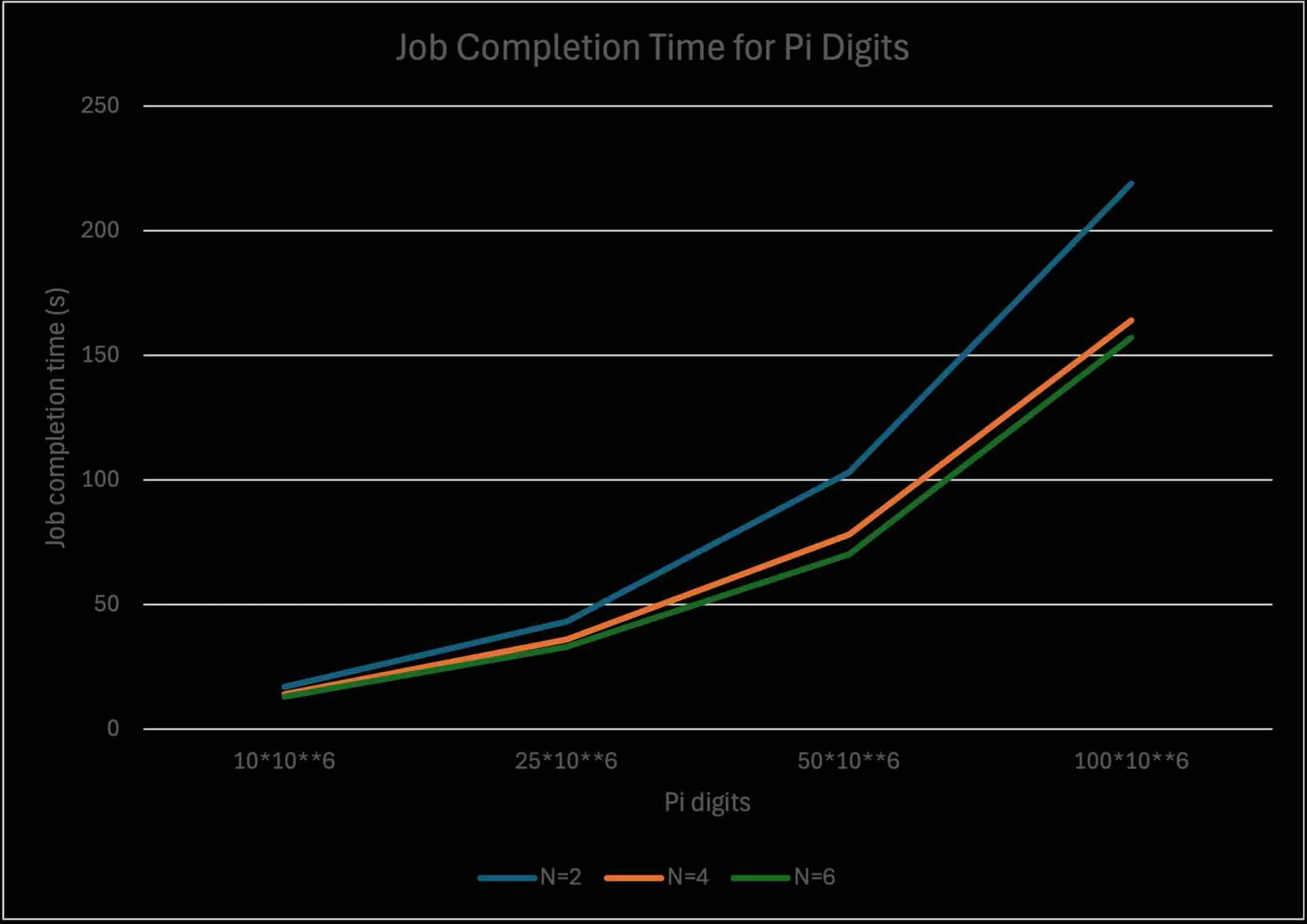
      controlledValues: "RequestsAndLimits"

The following graph shows the time to compute $\pi$ using 2, 4 or 6 replicas of the StatefulSet for 10M, 25M, 50M and 100M digits of $\pi$. The graph shows the increasing benefit of parallelism when the number of digits increases. Increasing the replica count beyond a certain number has lesser value since the time for combining the results coming from the StatefulSet pods to make the final computation to calculate the values of $a$ and $b$ for $\pi = \frac{426880\sqrt{10005}}{13591409a + 545140134b}$ becomes the more dominant part of the overall computation.

Complete the following steps for customization:

1. Create a namespace demo in your cluster.
2. Update $CONTENT/overlays/demo/kustomization.yaml to add the namespace and point to your container image registry for chudnovsky-worker and chudnovsky-merger.
3. Update $CONTENT/overlays/demo/pi-sets-demo.env, to set the number of $\pi$ digits, the number of steps (derived from dividing the number of $\pi$ digits by 14.18), the number of decimal digit per chunk when writing to the assigned volume.
4. Update $CONTENT/overlays/demo/pi-worker-statefulset-patch.yaml to set the count of replicas to be identical to WORKER_REPLICAS set in pi-sets-demo.env.
5. Adjust the values for the spec.resourcePolicy in the pi-worker-vpa-patch.yaml.
6. Run kustomize build $OVERLAYS/demo -o $RESOURCES to create all the resources.
7. Apply the resources one by one; wait for the completion of the merger Job and collect the digits of $\pi$ as stored in the mounted storage.

Blog’s lead image is 20,000 colored digits of $\pi$. Frequency of all digits are very similar whereas there are occasional interesting sequences. For example, digit ‘9’ is repeated 6 times starting at index 763.