Background

Prime numbers are fascinating. So fascinating that in an age when we are told (almost daily) that we are very close to the artificial super-intelligence, there are many unproven conjectures about prime numbers postulated more than 1000 years ago. Here is a simple one that is significantly newer.

For any natural number n greater than 1, there is at least one prime number between $n(n-1)$ and $n^2$; and similarly there is at least one prime number between $n^2$ and $n(n+1)$. You can even formulate it with less words and proper mathematical symbols: $\pi(n^2-n) < \pi(n^2) < \pi(n^2+n)$ where $\pi(x)$ is the number of prime numbers smaller than or equal to x.

Danish mathematician Ludvig Oppermann postulated the above conjecture in 1877. Like so many other interesting topics in number theory, it is related to the frequency of prime numbers in a given range of numbers. Closest anyone has ever come cracking the nut on that age old problem was German mathematician Riemann but even his most elegant formulation for calculating prime number frequency happens to be a hypothesis. I’d suggest to read an easy to read book Riemann Hypothesis: Greatest Unsolved Mathematics to get a better grasp of Prime Number Theory, Riemann, (in)famous zeta function $\zeta(x)$, and the frequency of prime numbers.

Going back to Oppermann’s conjecture, instead of trying to disprove the conjecture, i.e., trying to find an $n$ that doesn’t fulfill the inequality, a more interesting observation might be to count the number of primes in the lower range ($[n^2-n,n^2]$) and in the upper range ($[n^2,n^2+n]$) and compare them. Following graph is a plot to visualize for such comparison where the ratio of number of primes in the lower and upper ranges are included.

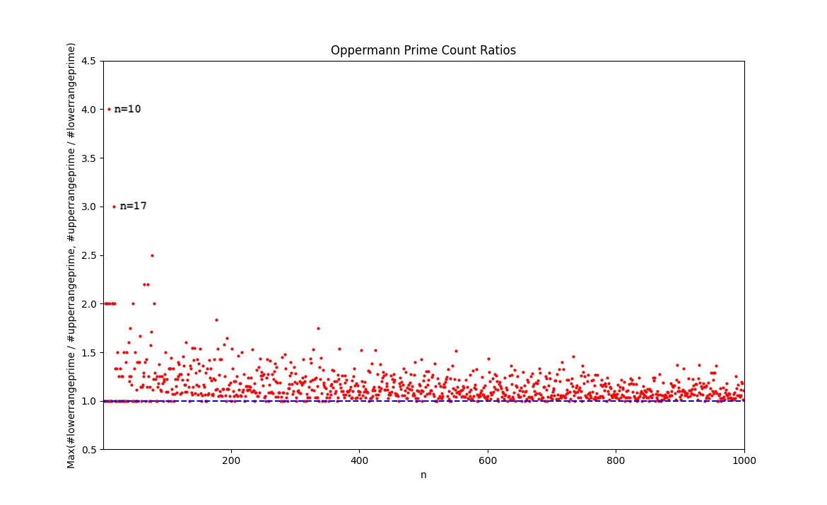
Just looking at this graph, one can quickly conclude that the number of primes in the range of [90,110] ({97}, {101, 103, 107, 109}) and in [272,306] ({277, 281, 283}, {293}) exhibit quite a significant imbalance. I might even be bold to make my own conjecture that the ratio of number of primes in the lower and upper ranges is always less than or equal to 4.

A more interesting characteristic might be to find numbers (let’s call them magic Oppermann, in short mO, numbers) such that around their square the distribution of prime numbers is very uniform. In other words for an mO number n will be such that $\pi(n^2)-\pi(n^2-n) = \pi(n^2+n)-\pi(n^2)$
Intuitively, we can observe that as n gets bigger its probability of being an mO number gets smaller since the range $[n^2-n,n^2]$ (or $[n^2,n^2+n]$) gets bigger. Leaving any conjectures around mO numbers aside, I plan to use the search for mO numbers for a fun exercise as described in the second part of this post.

Up to this point, I haven’t mentioned how I am finding which numbers are prime within a given range. When I originally started this exercise, I thought about using the Eratosthenes’ sieve as a fast way to calculate primality. Eratosthenes was a 3rd century BC math genius who happened to dabble in many things including measuring the Earth’s circumference. So called the sieve is a marvellous algorithm that avoids blind division tests but instead relies on multiplication to compute a list (more of a sieve) of prime numbers. If you are curious, please check the Wikipedia article Sieve of Eratosthenes. If you watch the animation on the Wiki page, you will understand how it works. One way to use the sieve is to pre-compute a sufficiently large sieve (with as many prime numbers as your memory allows you to store) and then use it for the division test. For the purpose of finding large mO numbers, the number of primality tests that need to be executed is 2n for a given n. Then we end up with two ways to check which numbers are mO numbers by checking which numbers are prime in the range of [N(N-1),N(N+1)]:

1. Pre-calculate all prime numbers less than $N$ using the Eratosthenes sieve and use the divisibility test. The cost in terms of memory is $k\pi(N)$ bytes while the cost in terms of operations is $2\pi(N)N$ divisions (assuming $N^2 >> N$).
2. Pre-calculate all prime numbers less than $N(N+1)$ using Eratosthenes sieve and perform a lookup. Cost in terms of memory is $k\pi(N(N+1))$ bytes while cost in terms of operations is $2N$ look-ups.

A clear trade-off between memory and computation manifests itself. Considering Python uses 28-bytes to represent a Boolean, the second approach requires other optimization techniques such as packing Boolean values into bit arrays. Such optimization methods end up having their own computational costs and introduce further complexity. Especially if your objective is to search for mO numbers in the ranges of $10^5$ or above in a reasonable amount of time without spending a lot of resources, you need to look for better methods than a 2300 year old algorithm.

Once I got into the territory of running primality tests for numbers in the vicinity of $10^{10}$ with my laptop, I realized I needed the help of better methods. Literature includes many faster probabilistic as well as deterministic algorithms including:

1. Fermat primality test
2. Miller-Rabin primality test
3. Solovay–Strassen primality test
4. Adleman–Pomerance–Rumely-Cohen-Lenstra primality test

(All of these were superseded by the amazing discovery of Agrawal–Kayal–Saxena primality test that is general, polynomial-time, deterministic, and not dependent on the Riemann hypothesis. Unfortunately for practical purposes, other tests such as APR-CL are proven to be more practical and that is why AKS test is not adopted in typical math software.)

When I started looking for code for some of these tests, I found out about SageMath, an open source mathematics software licensed under the GPL. SageMath can be used via an interactive command line, writing/compiling SageMath scripts, writing your own (Python) scripts that use the SageMath library, and using SageMath in Jupyter notebooks. It has a big set of libraries including those that I can use for fast primality tests.

The SageMath primality test can be called with the Boolean function, is_prime(). Using this function, following is an excerpt of calculating the number of primes in ranges $[n(n-1),n^2]$ and $[n^2,n(n+1)]$ for a given n:

def oppermann_prime_counts(n: int):
    if n < 2:
        print("Only natural numbers greater than 1 can be primes")
        return 0,0

    lower_range_primes = []
    upper_range_primes = []

    # we know n*(n-1) is always even, and we can skip even numbers for primality testing
    for i in range(n*(n-1)+1, n*n, 2):
        if is_prime(i):
            lower_range_primes.append(i)

    if (n*n)%2 == 0:
        a = 1
    else:
        a = 2

    # if n*n is even, we start testing from n*n+1, and we can skip even numbers for primality testing 
    for i in range(n*n+a, n*(n+1), 2):
        if is_prime(i):
            upper_range_primes.append(i)

    return len(lower_range_primes), len(upper_range_primes)

Alternatively we can use the $\pi(x)$ we saw earlier, along with the Legendre’s sieve for a more readable version:

def oppermann_prime_counts_with_legendre(n: int):
    if n < 2:
        print("Only natural numbers greater than 1 can be primes")
        return 0,0

    # p_pi: the number of prime numbers less than or equal to n
    p_pi = prime_pi(n)

    # legendre_phi(a, b) returns the number of numbers coprime to first b prime numbers
    return legendre_phi(n*n, p_pi) - legendre_phi(n*(n-1), p_pi), legendre_phi(n*(n+1), p_pi) - legendre_phi(n*n, p_pi)

SageMath can be installed as a binary for both Mac and Windows. Most of the Linux major distributions tend to have ~3 year old versions of SageMath that are deployable via their package managers (exceptions are Arch Linux and Void Linux). For both Mac and Linux, another appealing option is to deploy it from conda-forge using mamba or conda utilities. There is also a Docker image provided by CoCalc that offers a commercial product around SageMath. Ultimately, there is always the option of installing it from the source code.

Focus of Learning

My interest in all of this is to find interesting, easy to experiment with mathematical concepts that are explainable when I am learning how to use various technologies at a more proficient level. One example technology is Kubernetes, the well-adopted cloud-native workload orchestration tool. Kubernetes had its origins in an internal Google project that was open-sourced starting in 2014. For the last decade, it has seen more and more adoption and has become the de-facto technology choice if your ambition is to make your infrastructure cloud-provider agnostic and as programmable as your application code.

One of the basic Kubernetes primitives is Job that is equivalent to asynchronous and parallel execution paradigms found in object oriented programming languages. A Kubernetes Job triggers the instantion of a Pod (which is the nominal unit in Kubernetes to run a container), and upon successful execution of the task within the Pod it terminates. However, since it is not solely resident in the memory of an executable but written as part of the Kubernetes cluster’s resource database, it has multiple capabilities:

• it survives cluster restarts and node failures
• it is usable for tracking after completion
• it can be performed multiple times
• it provides a mechanism for parallel execution

There are two parameters defining the Job behavior:

• .spec.completions how many Pods must run to complete a job
• .spec.parallelism how many Pod replicas can run in parallel

.spec.completions	.spec.parallelism	Behavior
Unset (default 1)	Unset (default 1)	Single Pod Job
Set to number of completions	Optional	Fixed completion count Job
Unset (default 1)	Set to value > 1	Work queue Job

Fixed completion count Jobs can be made more elaborate by setting .spec.completionMode to Indexed, it is possible to have indexed Jobs that associate an index number (ranging from 0 to .spec.completions - 1) for each Pod of the Job. Such Jobs are useful for completing a pre-determined number of tasks based on a static work assignment and might be a topic for another blog in the future.

In this exercise, my plan is to use the work queue Job with the help of an external queue. For this purpose, I follow the example in Kubernetes docs fine parallel processing work queue that uses a Redis db.

Without getting into detailed praise of Redis, I can say that using it as a message queue looks very appealing to me. As highlighted in the Kubernetes documentation work queue example, retrieval of queue length via a Redis client is significantly simpler compared to advanced message queueing protocol of RabbitMQ. This allows inserting an arbitrary number of work items to a Redis db and allowing multiple Pods as triggered by the same Job to process those work items until the queue is depleted. Once all the Pods discover that there are no work items left to be processed they complete their execution and in turn Job is deemed to be completed.

Kubernetes docs example provides a set of files to complete the exercise including yaml templates for Redis Pod and Service, Job that triggers the creation of Pods, along with a Dockerfile and couple of Python scripts that describe the communication with the Redis db and the actual worker definition. Our job will be to amend the worker script to perform a search if a given number is an mO (magic Oppermann) number as I described earlier.

Before we start following the Kubernetes docs example, we need two essential components:

1. A Docker image that will be used in the Kubernetes Job
2. A Docker image that will be instantiated to provide the SageMath service via a REST API

Create a Container Image (for Customized Worker)

As described in the Kubernetes docs example, one essential task is to create a container image that is used to process the potential mO numbers. I used the Redis work queue client library (with all its TODOs), called rediswq.py as in the reference. I updated the worker.py and supplementing it with a SageMath API client library in sagemathapiclient.py.

I updated the Dockerfile of the Kubernetes docs example slightly to use python:slim image and use requirements.txt to add the relevant Python libraries.

Please refer to the GitHub repo oppermann-worker to build the Docker image and upload it to your own preferred Docker registry.

Create Another Container Image (for SageMath Backend)

My ambition was to have a portable SageMath instance that I can use in a Kubernetes environment. Since I didn’t have any success with downloading the CoCalc Docker images, I decided to build my own and I opted for using condaforge/miniforge3 as the base image. My other objective was to use SageMath behind a REST API to be able to use REST clients in various Kubernetes primitives. My choice for restification of SageMath was FastAPI, a REST framework that I was already familiar with.

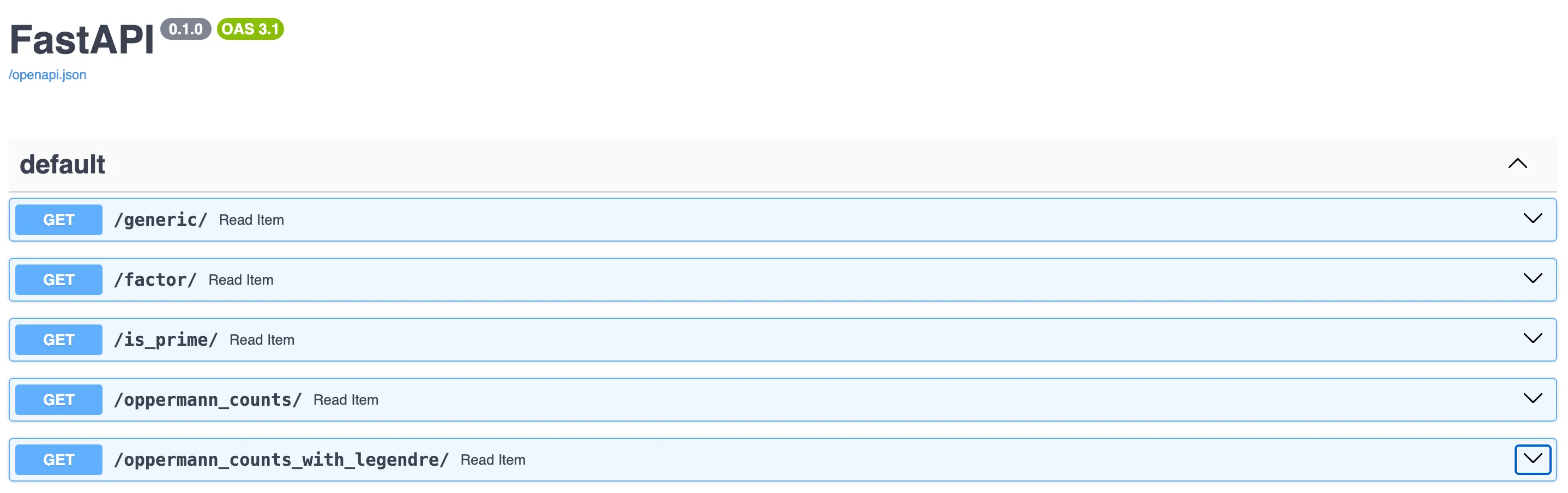
Using the FastAPI, I implemented few REST endpoints for the sample SageMath scripts that I generated for general interaction with SageMath as well as for calculating Oppermann numbers as I described earlier. For details, please check the git repository sagemath-backend-service. I’d recommend you adjust both the Dockerfile and the set of scripts as you prefer so that it is tailored for your execution environment. Here is a screenshot of the sample endpoints I used during this exercise.

Since I am running my Kubernetes cluster on small (10GB disk) VMs on my laptop, I opted to keep it running as a Podman container (> 9GB container image) on my laptop. That container was initiated by the following command:

podman run --rm -it -p 8000:8000 localhost/sagemath-backend-service:prime

Following Kubernetes docs Example

Assuming you happen to have access to a Kubernetes cluster, follow the instructions of the GitHub repo blog-prime-jobs to simplify the generation of resource files. I’d recommend you use the demo deployment option using kustomize.

Once you follow the installation instructions you will end up with a list of resources in your directory to be deployed similar to the following:

ls -l $RESOURCES
total 28
-rw-rw-r-- 1 ubuntu ubuntu 1218 Dec 18 11:06 batch_v1_job_mo-fill-job.yaml
-rw-rw-r-- 1 ubuntu ubuntu 1066 Dec 18 11:06 batch_v1_job_prime-job.yaml
-rw-rw-r-- 1 ubuntu ubuntu  311 Dec 18 11:06 discovery.k8s.io_v1_endpointslice_sagemath-service-endpointslice.yaml
-rw-rw-r-- 1 ubuntu ubuntu  293 Dec 18 11:06 v1_configmap_prime-job-environment-vars-6d9m6bgtkd.yaml
-rw-rw-r-- 1 ubuntu ubuntu  248 Dec 18 11:06 v1_pod_redis-master.yaml
-rw-rw-r-- 1 ubuntu ubuntu  194 Dec 18 11:06 v1_service_redis.yaml
-rw-rw-r-- 1 ubuntu ubuntu  288 Dec 18 11:06 v1_service_sagemath-service.yaml

Generating ConfigMap

Generate the configmap. In my case, I did:

kubectl apply -f v1_configmap_prime-job-environment-vars-6d9m6bgtkd.yaml

Starting Redis

Start a single instance of Redis, i.e, the Redis Pod and the Redis Service:

kubectl apply -f v1_pod_redis-master.yaml
kubectl apply -f v1_service_sagemath-service.yaml

Enabling SageMath Backend Service Accessible to Job

Since I ran the sagemath-backend-service external to the cluster, I created a headless Service named sagemath-service and the Endpoint Slice to make the REST API reachable from the Pods belonging to the Job. You need to adjust the spec.externalIPs in the sagemath-service-patch.yaml based on the IP address for the sagemath-backend-service:

  externalIPs:
  - 192.168.1.200

Also use the same value for the endpoints.addresses in the sagemath-endpointslice-patch.yaml:

endpoints:
- addresses:
  - "192.168.1.200"

Perform the following to enable access to the sagemath-backend-service:

kubectl apply -f v1_service_sagemath-service.yaml
kubectl apply -f discovery.k8s.io_v1_endpointslice_sagemath-service-endpointslice.yaml

Filling the Queue with Tasks

Instead of using the manual approach of the Kubernetes docs example, I used another job to fill it with integers. This Job is defined in mo-fill-job.yaml that can be customized with environment variables MO_START (starting point in the search for mO numbers), MO_COUNT (how many numbers to be searched), REDIS_SERVICE (name of the Kubernetes Service exposing the Redis db) and REDIS_QUEUE (name of the table used as the communication queue). All these variables are passed in a ConfigMap generated dynamically via kustomize.

kubectl apply -f batch_v1_job_mo-fill-job.yaml

You can always validate if the mo-fill-job successfully filled the database table by creating a temporary interactive Pod and using redis-cli commands.

kubectl -n demo run -it temp --image redis --command "/bin/sh"
If you don't see a command prompt, try pressing enter.

# redis-cli -h redis lrange job2 0 -1
  1) "100100"
  2) "100099"
  3) "100098"
  4) "100097"
...  

In case you want to re-initialize the table, simply flush the database and then run the mo-fill-job with a new set of environment variables.

# redis-cli -h redis flushdb
OK
# redis-cli -h redis lrange job1 0 -1
(empty array) 

About the Job Definition

For the Job definition, primary changes compared to the Kubernetes docs example are the inclusion of environment variables and the change in the restartPolicy. I added SAGEMATH_API_HOST and SAGEMATH_API_PORT to be able to use another Kubernetes service to access the REST API endpoint to collect Oppermann counts for a given integer. I modified the restartPolicy to be Never to prevent any issues that may arise due to uncompleted Redis db transactions that may be resolved if some of TODOs in the Redis work queue client library are completed.

Running the Job

As we have done all the preparations so far, the remaining task is to simply run the following command:

kubectl apply -f batch_v1_job_prime-job.yaml

Check the logs of the jobs that were completed:

kubectl -n demo get po
NAME                READY   STATUS      RESTARTS       AGE
prime-job-qsgs9      0/1     Completed   0              79s
prime-job-z6gmq      0/1     Completed   0              79s
mo-fill-job-b6k94   0/1     Completed   0              2m20s
redis-master        1/1     Running     0              4d20h
temp                1/1     Running     1 (3h5m ago)   3h20m
kubectl -n demo logs prime-job-qsgs9
Worker with sessionID: e6c62a6d-0df1-437c-8e57-f4b3f8712741
Initial queue state: empty=False
Waiting for work
Queue empty, exiting
kubectl -n demo logs prime-job-z6gmq
Worker with sessionID: d283ac4e-ddaf-4b47-a396-e261cef8ee91
Initial queue state: empty=False
1000132  yields a MAGIC with a pair of  36055  prime numbers on either side of its square.
Queue empty, exiting

Now thanks to this exercise, we know that 1000132 happens to be an mO number such that

$\pi(1000132^2) = \frac{\pi(1000132*1000131) + \pi(1000132*1000133)}{2}$

I will leave finding larger mO numbers to you as a fun exercise of what I have shared so far. Please download the code from blog-prime-jobs and run experiments as you wish. If you happen to find an mO number larger than 1000132, please drop me a note on your preferred choice of social media.

Blog’s lead image was generated from plotting primes (in yellow) and magic Oppermann numbers (in bright blue) less than 30000 in polar coordinates.