Background

If you are from my generation I am sure you will remember these lyrics and probably start humming as well:
With one breath
With one flow
You will know
Synchronicity
A sleep trance
A dream dance
A shared romance
Synchronicity

Sting wrote the song which also titled the Police album in 1983 as a tribute to The Roots of Coincidence by Arthur Koestler who borrowed the idea of Synchronicity from Carl Jung. Jung along with Wolfgang Pauli (that Nobel Physics prize winner) developed this pseudo-scientific idea about coincidental events typically between an internal thought or dream perfectly matching an external event in the world, even though one didn’t “cause” the other. Even to this day, there is a number of physicists, psychologists and science philosophers trying to find scientific meaning around the concept using quantum mechanics entanglement, quantum nature of conciousness, micro wormholes,… I am sure you got the idea.

On a more pedestrian side, synchronization which is the active coordination of two or more things to happen at the same time or rate is an easier concept to explain and experiment with. Synchronization occurs when two oscillators (events with a beat) that are connected by an external relationship eventually start having the identical beat. In this blog, I am going to cover the math behind synchronization as much as I understand and in the learning section use the opportunity to describe an almost real-life example to better understand custom resource definitions in Kubernetes.

Almost every article I looked at about synchronization starts with the experiments of Dutch scientist Christiaan Huygens in 1665. Huygens, who patented pendulum clock in 1656, observed two pendulum clocks starting to swing in unison (opposite directions) after a period of time irrespective of their starting positions while having an extended bed stay due to a sickness in February 1665. His rapid set of experiments triggered him to call this sympathy of two clocks and understand that the conformity of the rhythms of the clocks was caused by the difficult to observe movement of a beam where the two pendulums were hung. If you want to see the effect of such a common force in a more striking fashion, I’d recommend this video of 32 metronomes synchronizing.

Considering there are so many easy to observe natural synchronization phenomena, it is quite hard to believe until 1665 nobody articulated this properly. Well known examples include but not limited to:

• Male fireflies emit rythmic light pulses in order to attract females and they can synchronize their flashes with their neighbors. The blog’s lead image is a simulation of this.
• Male snowy tree crickets can synchronize their chirps by responding to the preceding chirps of their neighbors. It was shown that they can achieve synchronization in two cycles when the chirp rate is close to 200 per minute.
• Even humans are capable of such feat. Study from concerts in Romania and Hungary showed by even one individual reducing their frequency of clapping they can bring the whole audience to a synchronized rythmic hand clapping.

Synchronization can be collaborative as in the case of the listed examples. It can also be induced by an external force such as circadian rythms of humans and animals where the external force happens to be the daily cycle of light and dark. Synchronization can also apply to machines such as the phone or tablet where you may be reading this article so that the device knows when to listen the transmission of the base station or the access point that it is connected to. Similarly in computer, financial and industrial networks, devices ultimately derive their time reference from a time server. Such time servers themselves collect their references from a global navigation satellite system such as GPS. No wonder why one of the civilization level hazards of modern life is some solar storm that may wipe out GPS.

Before trying to formulate the synchronization, first let’s develop the description of the phenomena we are observing:

• Assume we have two oscillators, such as two fireflies blinking at frequencies $\omega_0$ and $\omega_1$.
• Assume with respect to some reference point in time, firefly-0 blinks $\phi_0$ seconds later while firefly-1 does the same $\phi_1$ seconds.
• Let’s also assume for the sake of simplicity that both fireflies have the same intensity, meaning the amplitude of their light is equal.
• Let’s also assume that they have the same pulse duration. In other words their light is ON for the same duration of time.
• Then the following formula can be written about our two fireflies lights

$F_0(t) = A\sum\limits_{k=-\infty}^{\infty}\delta(t - \frac{\phi_0+2\pi k}{\omega_0})$ and $F_1(t) = A\sum\limits_{k=-\infty}^{\infty}\delta(t - \frac{\phi_1+2\pi k}{\omega_1})$

In 1975 Yoshiki Kuramoto proposed a mathematical model to describe the synchronization of such oscillators. Without going into the details of the model, we can make the following observations about our two fireflies that are synchronizing their blinking:

• Imagine that two fireflies blinking is equivalent to the hand of a clock that is constantly moving in the clockwise direction. When the clock’s hand comes to the same position, the firefly blinks its light ON for a period of time (smaller than time it takes to get to the same clock position). Based on this description, let’s say firefly-0 phase is $\theta_0(t)$ and firefly-1 phase is $\theta_1(t)$.
• Their frequency of blinking is determined by the rate of change of their phase. In other words, $\frac{d\theta_0(t)}{dt} = \omega_0$ and $\frac{d\theta_1(t)}{dt} = \omega_1$.
• If they are not synchronizing, $\omega_0 \ne \omega_1$.
• In order to trigger the synchronization, there must be some force. In the case of fireflies, it is likely the evolutionary force that allow females to eliminate the noise to help them focus on the signal from males. Using this force, Kuramoto’s framework allows us to write the following equations: $\frac{d\theta_0(t)}{dt} = \omega_0 + Ksin(\theta_1 - \theta_0)$ and $\frac{d\theta_1(t)}{dt} = \omega_1 + Ksin(\theta_0 - \theta_1)$ where $sin(\theta_1 - \theta_0)$ acts as the correction signal and the value of K determines the strength of the coupling. In other words, higher the value of K, stonger the coupling and quicker the two fireflies get to synchronization.
• The perfect synchronization is achieved when $\theta_0 = \theta_1$ and the flashes occur when $\theta_0 = \theta_1 = 2\pi k$ which means when $t_k = \frac{\phi_i+2\pi k}{\omega_i}$ where $i = 0 | 1$.

You can extend this to multiple fireflies, pendelums or metronomes as you wish. My ambition is to look at something slightly different but a (close to) real life example that I will cover in the next section.

Focus of Learning

During the late 1980s, there was still an active debate about what computer networking protocols should look like. On one side number of international standardization bodies were actively pushing the so-called ISO stack. It had the support from all the world governments (including the US). On the other corner the TCP/IP stack with almost two decades of practical experience from ARPANET was trail-blazing with measurable improvements continuously. By early 1990s, the Internet based on the TCP/IP stack started becoming global and the contest was over. I took a graduate class on Computer Networks at that time thinking we would be covering this dichotomy and similar concepts. Instead, it turned out to be a great course on queueing theory. One of the questions the professor posed was as follows (including my paraphrasing):

• Suppose you have a circular track with N buses circling around it and there are M stations on the track uniformly distributed. Also assume that buses cannot pass each other but when one catches up with another they form a bus-convoy of two buses.
• Assume all buses travel at the speed of $v$ track-units/hour around the track.
• Passengers arrive at each station at the same rate $\lambda$ passengers/hour. When a bus arrives at a station, passengers get on at the rate $\mu$ passengers/hour. (Using the queueing theory parlance, both arrivals and loading are Poisson processes.)
• If we neglect the capacity of buses or stations; how long passengers stay on them and assume that at the initial state buses are uniformly distributed similar to the stations around the track, how long would it take for all these buses to form a single bus-convoy?

Here is a short video of a simulation of two buses chasing each other around a circular track.

After watching the video you must have realized the similarities between fireflies or metronomes synchronizing and buses forming a single convoy. In this case the external factor forcing the synchronization is the random differences in terms of the number of passengers arriving at each station. That randomness changes the dwell time for each bus at a station and allows eventually one bus to catch another. You can notice that more frequently a bus reaches a station, higher the chance of hitting a difference in the number of passengers awaiting compared to the other bus. Therefore, faster the buses travel, more likely they will encounter such difference and earlier they catch up each other. Similarly if we had more stations, we will encounter the same result of having a bus-convoy quicker.

Here are the results of few Monte Carlo simulations along with the analytical calculation for the probability of ending up with a single bus-convoy after T hours for various bus speeds.

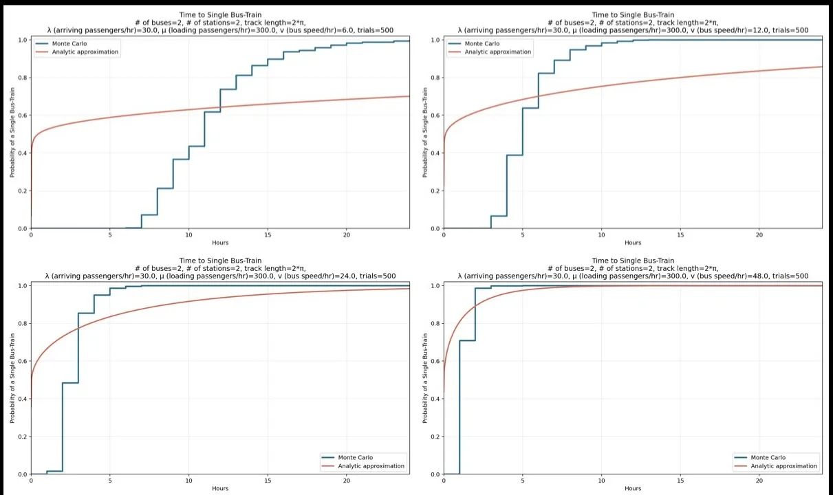
I am not going into the derivation of the analytical formula that requires its own article. Furthermore, I am not convinced what I have derived truly reflects the system. In other words, it needs further work.

Going back to the original plan of learning, I would like to use this system to take advantage of custom resource definitions construct of Kubernetes. The CustomResourceDefinition API resource allows extending the standard Kubernetes API with custom resources with a name and schema that users can specify. Going back to my synchronization example involving buses and stations, I can generate CRD objects corresponding to a bus simulation that would allow me to manipulate it in terms of allowed operations for buses, passengers, etc.

Implementation Details

In order to follow the rest of the blog, please check the GitHub repository blog-time-again.

Create a Container Image for Controller

This container image is implemented in Python using Kubernetes with the help of ChatGPT-5.4. Follow the instructions in the README file for the GitHub repository bus-passenger-controller to build and store the image. This image includes all the scripts for bus-passenger-controller Deployment.

Create a Container Image for UI

This container image is implemented in Python using FastAPI, Kubernetes as well as Javascript with the help of ChatGPT-5.4. Follow the instructions in the README file for the GitHub repository bus-passenger-ui to build and store the image. This image includes all the scripts for bus-passenger-ui Deployment.

Deployment of the Kubernetes Resources

Assuming you happen to have access to a Kubernetes cluster, follow the instructions of the GitHub repo blog-time-again to simplify the generation of resource files. I’d recommend you use the demo deployment option using kustomize.

Important part of this exercise is the ability to define a CRD and then create an instance of it to model the underlying physical world simulation. Here is the sample-bussimulation.yaml that can be kustomized as the initial state for the simulation.

apiVersion: demo.sync/v1alpha1
kind: BusSimulation
metadata:
  name: passenger-demo
spec:
  busCount: 18
  stationCount: 12
  epochDurationMinutes: 1
  arrivalRatePerMinute: 0.5
  boardingMinutesPerPassenger: 0.2
  speedPerMinute: 0.4
  paused: true
  resetNonce: 0

The simulation is executed by changing the state of the BusSimulation instance at every epoch. The UI collects the state and reflects it on the UI. If the user engages to change the parameters of the simulation, wants to restart or pause, those are performed by patching the BusSimulation instance.

Blog’s lead image was generated using the inspirational material from Nick Case on Fireflies.