Background

I fell in love with Vermeer’s paintings the first time I saw some of his (lesser importance) paintings at the Metropolitan Museum of Art in mid 1990s. Afterwards I have read books, watched movies about the mysterious Dutch painter. Visiting Mauritshuis Museum in Amsterdam and seeing the Girl With a Pearl Earring before the Instagram era was a delight.

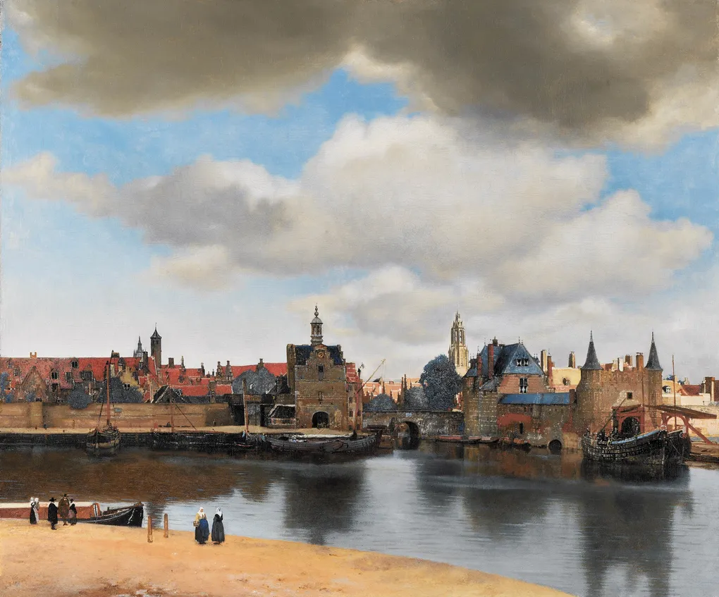
Recently I read this article about a research project on when Vermeer painted A View of Delft (the blog’s lead image) while looking for Vermeer paintings. Research team from the Texas State University looked at multiple clues including the coordinates of the estimated vantage point, light/shadow in the painting, historical records about the buildings in the painting, leaves on the trees and estimated that Vermeer painted the scenery as he saw it from the second floor of a 17th century inn on either September 3rd or 4th, 1659 at 8 am in the morning. I think the claim of accuracy is extraordinary and it certainly needs an extraordinary proof but I am not here to try refuting their work. Instead, I thought about how to develop a similar prediction tool for a given image if the exact coordinates of its vantage point are known.

Such a predictor could be useful to detect counterfeit (these days AI-generated) images with wrong claims about location or time when they were taken. Considering the significant cost involved in the detection, it is quite unlikely that the run-of-the-mill image generators will be able to achieve high fidelity for a while.

The practice of identifying the time window for a given image is part and parcel for Open Source Intelligence (OSINT) framework. It is referred as chronolocation. The general idea is based on the known location of the image, identify visible features that are temporal such as shadow (presence, direction, length), leaves (presence, color), ground cover (snow), human-made landmarks (presence, shape), etc. and compare them against known (time and location) images with similar features. For my quick experiment I decided to stick to the very basic shadow analysis. When I had limited success with that I tried to enrich it with some visual language model assistance that I will summarize at the end of the blog.

Focus of Learning

There are two essential components used in the time-of-day and day-of-year prediction based on shadow analysis:

• Estimate shadow direction from the image
• Generate the set of sun azimuth and elevation figures for a given latitude/longitude

It sounds pretty simple but in practice it has a set of intricacies. Before delving into each, let’s set the framework.

Image Coordinates

Let the image coordinate system be:

• $x$ : horizontal pixel coordinate, increasing to the right
• $y$ : vertical pixel coordinate, increasing downward

A cast shadow in the image is approximated by a line segment.

If a detected line segment has endpoints:

• $(x_1, y_1)$
• $(x_2, y_2)$

then its direction vector is:

$v = (dx, dy) = (x_2 - x_1, y_2 - y_1)$

The segment angle can be written with $atan2()$ function:

$\theta = atan2(dy, dx)$

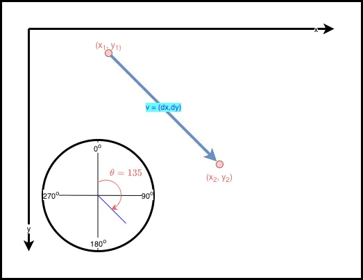
For the sake of code development, it is often more convenient to express angle clockwise from image up (negative y-axis in the diagram) rather than from the positive x-axis. A common conversion is:

$\theta = (degrees(atan2(dx, -dy)) + 360) mod 360$

This makes $\theta$ as:

• 0° near image up
• 90° near image right
• 180° near image down
• 270° near image left

Edge Detection

As mentioned earlier, the first goal in the chronolocation predictor is to generate the shadow lines from a given image. However, the typical image is full of noise and has limited contrast. This is why it is recommended to use an edge detector to generate a binary edge map that would be used by a transformer that would detect lines.

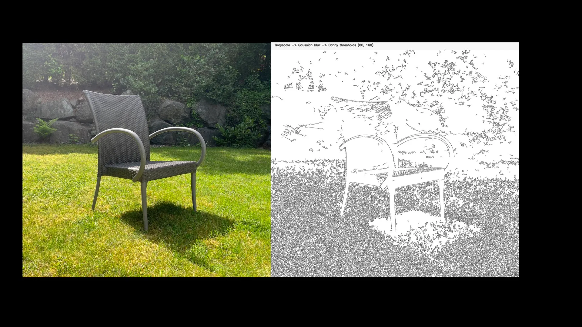
A good example is Canny edge detector that was developed by John F Canny. It works on a grayscale image that was blurred (to reduce noise). It is based on the idea of finding the intensity gradient of an image. Numerous edge detection methods would return the derivative of the change in pixel intensity in x and y directions to supply the Canny edge detector. Following is an example image and its computed edges.

Probabilistic Hough Line Transform

History of Hough transform is a great article that describes the progression of Hough transform from the original patent to the widely used method to detect lines in images.

The basic idea of the Hough transform is to calculate all possible lines that can pass through a point and find the lines that the most points can belong to. It sounds simple but it was quite an amazing feat to reformulate the problem into basic trigonometry and algebra.

Let’s take a look at a simple drawing from the same article (re-drawn for clarification) to better understand the transform method.

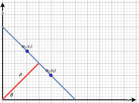
The blue line in the drawing passing through $(x_1, y_1)$ and $(x_2, y_2)$ can be rewritten as:

$\rho = x cos(\theta) + y sin(\theta)$

where:

• $\rho$ is the perpendicular distance from the origin
• $\theta$ is the line normal angle measured from the x-axis

Now, let’s look back at the equation for $\rho$ and plot it for few points on the blue line. In this plot the x-axis is $\theta$ and the y-axis is $\rho$.

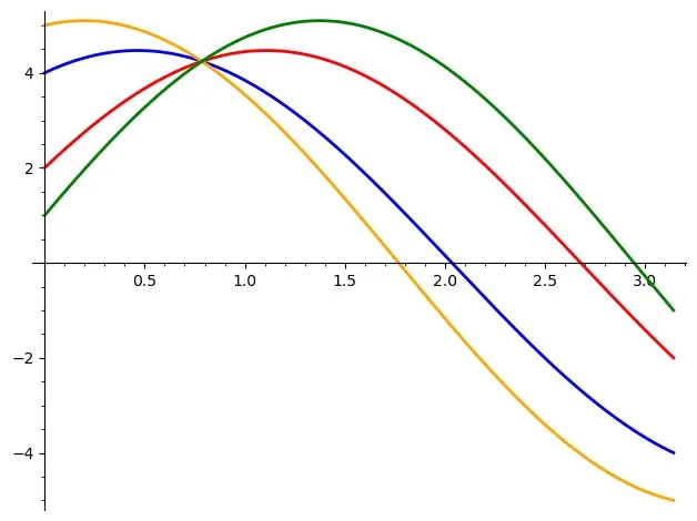
Each sinusoid in this graph shows all the possible combinations of $(\theta, \rho)$ for a given point $(x,y)$ on the original image for $0 \lt \theta \lt \pi$. For the selected points, the sinusoids intersect at $(\frac{\pi}{4}, 3\sqrt{2})$.

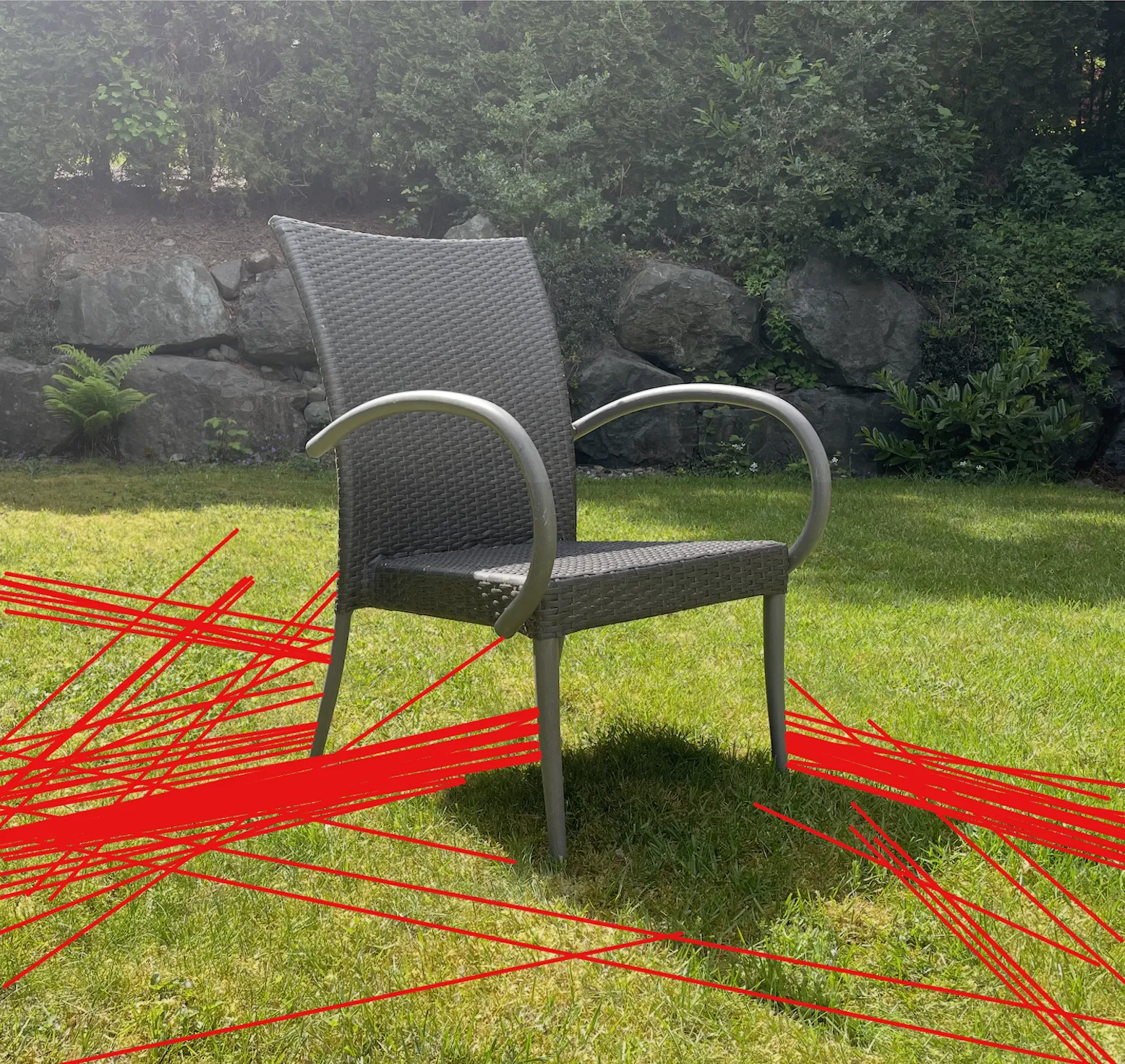
Using this methodology and selecting points from the output of the edge detector, the probabilistic Hough transform returns sampled line segments: $(x_1, y_1, x_2, y_2)$ These segments are candidate shadow or structure (such as a road or the edge of a building) lines.

The following figure shows a subset of the candidate shadow lines for the earlier test image.

Both for Canny edge detection and probabilistic Hough line generation, I relied on the OpenCV library. OpenCV has been the primary computer vision library since its first release in 2000. It has 2500+ algorithms and integration with machine learning libraries that allow expansion of traditional computer vision with statistical inference capabilties.

Heuristic Selection of Shadow Lines

A simple heuristics was used to prefer likely ground-shadow lines, for example:

• prefer segments in the lower part of the image
• prefer longer segments
• reject near-vertical clutter or skyline edges
• aggregate multiple segments instead of trusting one segment alone

Assume $N$ line segments with image-space unit direction vectors: $u_i = v_i / |v_i|$ and weights $w_i$ are selected based on segment length and location.

Using these definitions, the weighted average dominant shadow direction for an image becomes: $u_{avg} = \frac{\sum\limits_{i=1}^{N} w_iu_i}{|\sum\limits_{i=1}^{N} w_iu_i|}$

Then the sun direction is estimated to be $180^o$ opposite of the dominant shadow direction.

In order to estimate the sun elevation, the likely clues are shadow strength and the constrast of the image. Using these as heuristics, it is possible to generate a qualification such as low, medium, high for the sun elevation.

Candidates for Sun Azimuth and Elevation

Once how to generate the sun direction and a class for the sun elevation for a given image are understood, the remaining step in the predictor is generating a set of candidates for the sun azimuth and elevation for a given location (latitude, longitude). For this purpose, there are a number of open source tools available. In this experiment, I used pvlib. Pvlib was developed by solar energy enthusiasts to simulate solar energy systems. It provides methods to generate the sun azimuth and elevation for a given location at a given time. Using pvlib, you can generate a set of sun azimuth and elevation values, compare them against the results of the shadow line analysis, select a pre-determined number and present them to the user along with its calculated confidence.

Implementation Details

In order to follow the rest of the blog, please check the GitHub repository blog-timeless-images. All the code listed in the repo have been developed by Codex (GPT 5.4). My contribution was to supply prompts, supply test data, run tests, and try out various hypotheses.

As mentioned in the README, you can run the code locally (by setting a virtual environment). I would strongly recommend you run a benchmark as well. For that purpose, place as many files as you would like in the benchmark/raw directory. Assuming these files have location and camera direction information, follow the instructions below to generate first the ground truth dataset.

source .venv/bin/activate
python -m benchmark.build_dataset   --raw benchmark/raw   --out benchmark/testdata   --ground-truth benchmark/ground_truth.json   --force

To run the benchmark locally against the direct inference function:

python -m benchmark.run   --ground-truth benchmark/ground_truth.json   --testdata benchmark/testdata   --out benchmark/results/benchmark_results.csv

This writes:

• benchmark/results/benchmark_results.csv
• benchmark/results/benchmark_results.json

If you want to generate the production version, simply generate a container and run it.

podman build -t chronolocation .
podman run --rm -p 8000:8000 chronolocation

Lessons Learned

The predictor using the shadow direction estimate and pattern-matching that brute-force generated sun azimuth and elevation figures is entirely deterministic and has not been “trained” or “adjusted” using any large datasets. Instead I skimmed through some photos I’ve accumulated through years and selected 90 for benchmarking.

Benchmark summary of the predictor I shared for my dataset is as follows.

Out of 90 images	Elevation error $\lt$ 9o	9o $\le$ Elevation error $\lt$ 30o	Elevation error $\ge$ 30o
Azimuth error $\lt$ 18o	$\color{green}{\text{8}}$	$\color{yellow}{\text{5}}$	$\color{red}{\text{8}}$
18o $\le$ Azimuth error $\lt$ 60o	$\color{yellow}{\text{3}}$	$\color{yellow}{\text{11}}$	$\color{red}{\text{21}}$
Azimuth error $\ge$ 60o	$\color{red}{\text{5}}$	$\color{red}{\text{10}}$	$\color{red}{\text{19}}$

I chose threshold targets of $9^o$ and $30^o$ for the sun elevation while for the sun azimuth I picked $18^o$ and $60^o$. My ambition was to keep the both azimuth and elevation errors of 10% of the maximum values. As the table shows, this untrained/unadjusted predictor has quite limited accuracy. Less than 10% of the tested images were predicted with less than 10% error in both azimuth and elevation.

The Hough-line method has several structural weaknesses:

• it confused shadows with roads, horizons, railings, and other linear edges
• it had no true notion of ground plane or vertical shapes
• it only had a coarse elevation classifier
• it could not use semantic signals like snow, leaf state, clothing, or activity patterns

There are few ideas to experiment with to improve the prediction accuracy:

1. Replace Hough-line shadow detection with segmentation for ground plane, shadows, and vertical shapes that are creating the shadows.
2. Replace the coarse elevation classifier with a learned estimator using horizon line, shadow length, and sky radiance cues.
3. Add a scene-understanding model to provide semantic clues.

I have done some of those tests including performing some local ML model development for a learned coarse elevation estimator. I didn’t go to trouble of adding any further labeling but I also experimented with a local LLaVA model to see how good its scene description capabilities are. Without going into any details, I can say the amount of improvements based on these experiments were all limited. They were not consistent across all image types and scenes. If you are interested in finding out any details about those experiments please reach out on one of the social media links in the header.

My final test for each predictor was Vermeer’s painting of Delft. I uploaded a screenshot of the painting along with the coordinates of the Vermeer’s estimated vantage point (52.0046, 4.3612) and the camera direction ($338^o$) I estimated based on Google Maps. Likely by pure coincidence, the predictor’s results (at least one of its top 10) matched exactly one of the Texas State research team’s estimates: April 8th, 07:00-07:40. They also did contextual analysis and due to the presence of leaves, they ruled out the April date and settled on September 3-4 that is equivalent in terms of the sun direction. What pleased me was the consistency of the sun direction ($80.6^o$) and a small range for the sun elevation of the predictor results. Perhaps at least for some photos, this predictor could be a starting point to develop something more robust in the future.

Blog’s lead image is By Johannes Vermeer - www.mauritshuis.nl : Home : Info : : Image, Public Domain A View of Delft.